Sixth researcher

Discovering tumor neoantigens is easier than getting a job in Spain

November 13, 2017 / Alvaro Sebastian / 5 Comments

The story of this post started few months ago at a immunotherapies conference in Barcelona, at this time I was looking for a job in cancer research. I had a great time learning about new cancer therapies and meeting nice people, but few doctors were interested, or had money, to contract a bioinformatician. Nevertheless, one of them told me: “I don’t know you, but if you show me that you are able to discover tumor neoantigens, then I’ll consider to contract you in the future”. I hope this person will read the post 😉

But before starting, I want to dedicate this post to all the doctors, nurses, scientists and patients that fight everyday against cancer, specially those from Hospital Miguel Servet de Zaragoza and Clínica Universidad de Navarra that treat my father, also to many other brilliant and devoted people that I have met from places like Vall d’Hebron Hospital, Quiron Dexeus or 12 de Octubre, and finally, to my new team at Agenus Pharmaceuticals.

State of the art of tumor neoantigen discovery

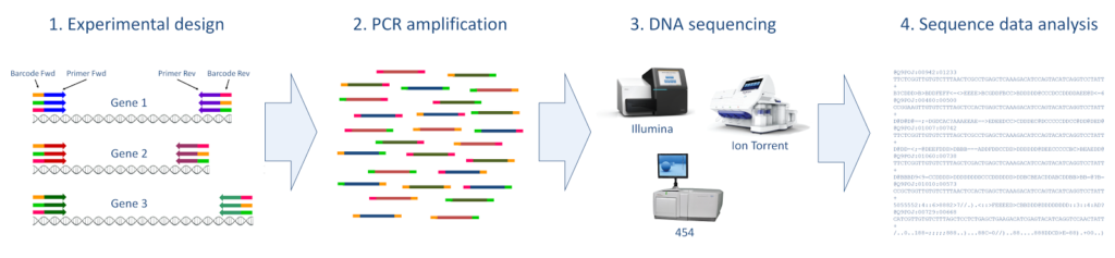
With next generation sequencing (NGS) we are able to sequence the full genome of a tumor or at least of the coding regions or exome. If we identify with the help of NGS data which tumor-specific genes express mutant peptides that are able to activate T cells, then we can design vaccines to boost the natural immune response to the tumor, this mutant peptides are also called neoantigens. There is a nice and recent Nature Review about neoantigens discovery, and also there are interesting articles with practical cases of neoantigens discovery and personalize treatments for cancer patients (e.g. Robbins et al., Pritchard et al.).

But we are interested in the bioinformatics point of view, so let’s make a summary of some neoantigens discovery protocols and software in the literature:

pVAC-Seq v4.0: a pipeline for the identification of personalized Variant Antigens by Cancer Sequencing (pVAC-Seq) that integrates tumor mutation and expression data (DNA- and RNA-Seq) (original article).
TSNAD: an integrated software for cancer somatic mutation and tumour-specific neoantigen detection (original article).
neoantigenR: an R package that identifies peptide epitope candidates (biorxir article).
MuPeXI: mutant peptide extractor and informer, a tool for predicting neo-epitopes from tumor sequencing data (original article).
INTEGRATE-neo: a pipeline for personalized gene fusion neoantigen discovery (original article).

We can conclude that the topic is quite new, most of the previous pipelines have been published during the last year, and that the neoantigen identification is a very complex task as we can see for example in the pVAC-Seq workflow schema:

Overview of the pipeline pVAC-Seq

To show an example of neoantigens discovery pipeline, I’ll try to simplify the process and follow the Best Practices guide from The Broad Institute for somatic variants discovery:

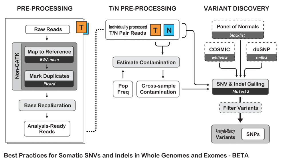
Best Practices for Somatic SNV and Indel Discovery

Tumor neoantigen discovery pipeline description

This protocol has been developed for didactic purposes and it is not formally validated neither intended for human diagnosis.

Basically I propose here a somatic variant calling pipeline with some additional filtering of the variants at the end. I tested the pipeline with whole exome sequencing (WES) Illumina paired-end reads from normal and tumor tissues.

The full pipeline can be summarized in 10 steps, here is briefly explanation of every step and some additional considerations about the chosen tools:

Normal and tumor reads mapping, sorting and indexing:
- In the protocol I have chosen BWA-MEM as recommended in Cornish and Guda paper, original authors used Novoalign, but other aligners could be considered. In this aspect, aligners as Bowtie2 may be too sensitive and could report some extra false positive variants, but it’s just a personal opinion.
Removal of duplicated reads:
- Maybe this step could be skipped as there are not many redundant reads and it’s unlikely that they map in variant positions. MarkDuplicates from Picard tools was used, I would suggest in the future to try ‘MarkDuplicatesWithMateCigar’ from the same suite, but I have not enough experience to recommend it.
Adding sample/group information to the mapped reads:
- This is just a formal requirement for the variant callers to work properly and distinguish between normal and tumor groups of reads.
Realignment around indels:
- This step is already integrated in the Mutect2 somatic variant caller and could be redundant, but other variant callers do not integrate it so it is strictly recommended to avoid false calling of indels and surrounding SNPs.
Somatic variant calling with MuTect2:
- MuTect2 is integrated in the GATK suite, the basic operation of MuTect2 proceeds similarly to that of the popular HaplotypeCaller, with a few key differences, taking as input tumor and normal alignments and producing somatic variant calls only.
Filtering of somatic variants:
- Some strict filters are imposed to discover only true somatic variants: a minimum depth of 10 reads and a variant frequency of at least 10%. Additionally, variants must be in coding regions of genes (it is filtered in the last step).
Annotation of filtered somatic variants
- Filtered variants are annotated: gene and transcript names and IDs, chromosome position, nucleotide and protein mutations and other relevant information about the antigens is annotated in a tabulated, CSV or HTML human readable format
Neoantigen peptides design
- Neoantigen peptides are designed extracting the amino acid sequence containing the variant (10-15 residues)
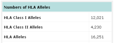
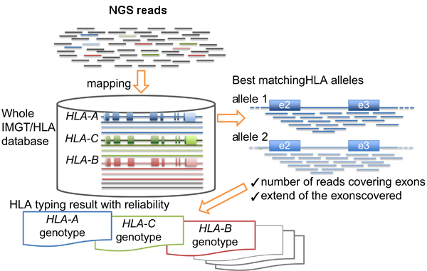
HLA-typing with exome or RNA-seq data
- Normal and tumor or RNA-seq (more accurate) data will be used as input of AmpliHLA to retrieve the HLA alleles of the patient.
HLA-binding affinity calculation and peptide ranking
- NetMHCpan software will calculate the binding affinities of the designed peptides to HLA alleles, these predictions together with expression data will be used to estimate the potential immunogenicity of the peptides.

Required tools and files

Before starting, you should install in your server or computer the following tools:

BWA aligner
SAMtools
VCFtools
Picard
GATK 3.8 (GATK4 is still not functional)
Variant filtering scripts
AmpliHLA
NetMHCpan

And download human genome files and SNP/indels annotations (be always consistent with the genome version and have in mind that new versions could be available):

Human genome in FASTA format (e.g. Homo_sapiens.GRCh38.dna.primary_assembly.fa.gz)
Human curated indel database (e.g. Mills_and_1000G_gold_standard.indels.b38.primary_assembly.vcf.gz)
The Single Nucleotide Polymorphism database (dbSNP, e.g. All_20170710.vcf.gz)
The Catalogue Of Somatic Mutations In Cancer (COSMIC, e.g. CosmicCodingMuts.vcf.gz)

Previous files (or equivalent ones) can be also downloaded from Google Cloud repository (not tested).

After this long introduction, let’s start the analysis…

Somatic variant calling and tumor neoantigen discovery pipeline

To simplify I’ll consider that all the input files, including the genome and reads ones, are in the working directory and all the output files will be stored into the ‘output’ folder. All the comments are marked with ‘#’ to differentiate them from the commands. Programs will be installed in the standard ‘/opt’ folder in the Linux system and run with 30 threads when it is possible (number of parallel threads/processes should be adjusted depending of your server or computer). Analysis time will depend of the system and the number of parallel processes, in a small server with 30 threads it may take around 15-20 hours to be completed. Steps 8 and 10 are sill not fully automatized.

1. Normal and tumor reads mapping, sorting and indexing

# Index genome FASTA file for BWA mapping:
/opt/bwa-0.7.15/bwa index Homo_sapiens.GRCh38.dna.primary_assembly.fa

# Normal reads mapping, sorting and indexing with BWA-MEM:
/opt/bwa-0.7.15/bwa mem -M -v 1 -t 30 Homo_sapiens.GRCh38.dna.primary_assembly.fa NORMAL_R1.fastq.gz NORMAL_R2.fastq.gz | /opt/samtools-1.6/bin/samtools view -Sb -F 4 -@ 30 | /opt/samtools-1.6/bin/samtools sort -@ 30 > output/NORMAL.bam ; /opt/samtools-1.6/bin/samtools index -@ 30 output/NORMAL.bam output/NORMAL.bai
# Tumor reads mapping, sorting and indexing:
/opt/bwa-0.7.15/bwa mem -M -v 1 -t 30 Homo_sapiens.GRCh38.dna.primary_assembly.fa TUMOR_R1.fastq.gz TUMOR_R2.fastq.gz | /opt/samtools-1.6/bin/samtools view -Sb -F 4 -@ 30 | /opt/samtools-1.6/bin/samtools sort -@ 30 > output/TUMOR.bam ; /opt/samtools-1.6/bin/samtools index -@ 30 output/TUMOR.bam output/TUMOR.bai

2. Removal of duplicated reads

# Removes normal duplicated reads:
java -jar /opt/picard-2.14.0/build/libs/picard.jar MarkDuplicates VERBOSITY=ERROR VALIDATION_STRINGENCY=SILENT REMOVE_DUPLICATES=true I=output/NORMAL.bam O=output/NORMAL.dups_removed.bam M=output/NORMAL.metrics.txt
# Removes tumor duplicated reads:
java -jar /opt/picard-2.14.0/build/libs/picard.jar MarkDuplicates VERBOSITY=ERROR VALIDATION_STRINGENCY=SILENT REMOVE_DUPLICATES=true I=output/TUMOR.bam O=output/TUMOR.dups_removed.bam M=output/TUMOR.metrics.txt

3. Adding sample/group information to the mapped reads

# Adds normal read group, the name of the individual and the phenotype (3998_normal):
java -jar /opt/picard-2.14.0/build/libs/picard.jar AddOrReplaceReadGroups VERBOSITY=ERROR VALIDATION_STRINGENCY=SILENT CREATE_INDEX=true SO=coordinate RGID=3998_normal RGLB=3998_normal RGPL=illumina RGPU=3998_normal RGSM=3998_normal I=output/NORMAL.dups_removed.bam O=output/NORMAL.grouped.bam
# Adds tumor read group, the name of the individual and the phenotype (3998_tumor):
java -jar /opt/picard-2.14.0/build/libs/picard.jar AddOrReplaceReadGroups VERBOSITY=ERROR VALIDATION_STRINGENCY=SILENT CREATE_INDEX=true SO=coordinate RGID=3998_tumor RGLB=3998_tumor RGPL=illumina RGPU=3998_tumor RGSM=3998_tumor I=output/TUMOR.dups_removed.bam O=output/TUMOR.grouped.bam

4. Realignment around indels

# Normal reads realignment around indels using the GATK modules RealignerTargetCreator and IndelRealigner:
java -jar /opt/gatk-3.8/GenomeAnalysisTK.jar -T RealignerTargetCreator -nt 30 -R Homo_sapiens.GRCh38.dna.primary_assembly.fa -I output/NORMAL.grouped.bam -known /Mills_and_1000G_gold_standard.indels.b38.primary_assembly.vcf.gz -o output/NORMAL.intervals ; java -jar /opt/gatk-3.8/GenomeAnalysisTK.jar -T IndelRealigner -maxReads 100000 -maxInMemory 1000000 -R Homo_sapiens.GRCh38.dna.primary_assembly.fa -targetIntervals output/NORMAL.intervals -I output/NORMAL.grouped.bam -known /Mills_and_1000G_gold_standard.indels.b38.primary_assembly.vcf.gz -o output/NORMAL.realign.bam
# Tumor reads realignment around indels using the GATK modules RealignerTargetCreator and IndelRealigner:
java -jar /opt/gatk-3.8/GenomeAnalysisTK.jar -T RealignerTargetCreator -nt 30 -R Homo_sapiens.GRCh38.dna.primary_assembly.fa -I output/TUMOR.grouped.bam -known /Mills_and_1000G_gold_standard.indels.b38.primary_assembly.vcf.gz -o output/TUMOR.intervals ; java -jar /opt/gatk-3.8/GenomeAnalysisTK.jar -T IndelRealigner -maxReads 100000 -maxInMemory 1000000 -R Homo_sapiens.GRCh38.dna.primary_assembly.fa -targetIntervals output/TUMOR.intervals -I output/TUMOR.grouped.bam -known /Mills_and_1000G_gold_standard.indels.b38.primary_assembly.vcf.gz -o output/TUMOR.realign.bam

5. Somatic variant calling with Mutect2 (GATK tool)

# Creates dbSNP VCF index file required by GATK:
gunzip /All_20170710.vcf.gz ; bgzip /All_20170710.vcf ; tabix -p vcf /All_20170710.vcf.gz
# Base quality score recalibration for normal reads alignments (BQSR):
java -jar /opt/gatk-3.8/GenomeAnalysisTK.jar -T BaseRecalibrator -nct 30 -knownSites /All_20170710.vcf.gz -R Homo_sapiens.GRCh38.dna.primary_assembly.fa -I output/NORMAL.realign.bam -o output/NORMAL.bqsr ; java -jar /opt/gatk-3.8/GenomeAnalysisTK.jar -T PrintReads -nct 30 -BQSR output/NORMAL.bqsr -R Homo_sapiens.GRCh38.dna.primary_assembly.fa -I output/NORMAL.realign.bam -o output/NORMAL.recalib.bam
# Base quality score recalibration for tumor reads alignments (BQSR):
java -jar /opt/gatk-3.8/GenomeAnalysisTK.jar -T BaseRecalibrator -nct 30 -knownSites /All_20170710.vcf.gz -R Homo_sapiens.GRCh38.dna.primary_assembly.fa -I output/TUMOR.realign.bam -o output/TUMOR.bqsr ; java -jar /opt/gatk-3.8/GenomeAnalysisTK.jar -T PrintReads -nct 30 -BQSR output/TUMOR.bqsr -R Homo_sapiens.GRCh38.dna.primary_assembly.fa -I output/TUMOR.realign.bam -o output/TUMOR.recalib.bam

# Calls somatic variants (SNPs and indels) via local re-assembly of haplotypes with MuTect2:
java -jar /opt/gatk-3.8/GenomeAnalysisTK.jar -T MuTect2 -nct 30 -D /All_20170710.vcf.gz -cosmic /CosmicCodingMuts.vcf.gz -R Homo_sapiens.GRCh38.dna.primary_assembly.fa -I:normal output/NORMAL.recalib.bam -I:tumor output/TUMOR.recalib.bam -o output/normal_vs_tumor.mutect2.all.vcf

6. Filtering of somatic variants

MuTect2 may retrieve more than 10000 variants, but after filtering the number is reduced around 8-10 times.

# Filters somatic variants called by each method:
filter_somatic_variants.pl -pass -vardepth 10 -varfreq 0.1 -i output/normal_vs_tumor.mutect2.all.vcf -o output/normal_vs_tumor.mutect2.somatic.vcf

7. Annotation of filtered somatic variants

If we obtained around 1000 variants after previous filtering step, the annotation of only variants present in coding regions will reduce the number to few hundreds.

# Annotates final variants and prints the details in a tabulated format file:
annotate_variants.pl -i output/normal_vs_tumor.mutect2.somatic.vcf > output/normal_vs_tumor.mutect2.somatic.txt

8. Neoantigen peptides design

# Creates a FASTA file with the sequences of the peptides (13 aa) containing the somatic mutations previously detected
variants_to_peptides.pl -l 13 -i output/normal_vs_tumor.mutect2.somatic.vcf -o output/normal_vs_tumor.mutect2.peptides.fa

9. HLA-typing with exome or RNA-seq data

# Analyzes WES, or RNA-seq if available, data and retrieves the HLA alleles of the patient that will be used in the last step to calculate the affinities of the peptides.
ampliHLA.pl -thr 30 -ty mapping -r gen -i NORMAL_R1.fastq.gz NORMAL_R2.fastq.gz > amplihla_normal.txt
ampliHLA.pl -thr 30 -ty mapping -r gen -i TUMOR_R1.fastq.gz TUMOR_R2.fastq.gz > amplihla_tumor.txt

10. HLA-binding affinity calculation and peptide rankin

# Calculates and ranks the MHC-binding affinity
netMHCpan -BA -xls -f output/normal_vs_tumor.mutect2.peptides.fa -a HLA-A01:01,HLA-A02:01,HLA-B15:01...

Finally I didn’t get any job in Spain, but I learned a lot 🙂

When students outperform their teacher – Part 1

March 23, 2017 / Alvaro Sebastian / 0 Comments

This post is a tribute to the work of my students in the subject “Basic Python Programming for Scientists“, as they did a great job in their final projects I want to show you here some examples that could be useful for many Python beginners. Remember that you can download the course slides from Didactic Materials sections.

First of all, I want so say that it was my first experience as Python Programming teacher and I was gratefully surprised with my students. I have learned a lot with them and I can say that some of them outperformed the teacher. I also want to thank to Medhat Helmy and Piotr Bentkowski for helping me in the teaching task. Unfortunately I cannot have the same opinion from the Adam Mickiewicz University that didn’t pay me any money for teaching, welcome to Poland…

Today I’ll show you 2 projects that overcame all my expectations: Image Quiz from Błażej Szymański and Temperature converter by Michal Stachowiak.. In next days I’ll publish more incredible projects.

Image Quiz

Click to play Image Quiz online

Maybe the project that impressed me the most was ‘Image Quiz’ by Błażej Szymański. He was planning at the beginning to write a python script that automatically downloads different airplane model images from Google, and later use these images with an HTML+JavaScript interface to play a quiz to guess which is the correct airplane model shown in a randomly selected image. I suggested some minor changes, like using a more biological topic as bird species instead of airplanes. And now you can check yourself the final result playing the Image Quiz online!

The project consists basically in 4 python scripts:

fetcher.py: reads a file ‘list.txt’ containing the names of the birds to look for and use the Google API to retrieve the bird photo URLs that are stored as JSON format in ‘data.txt’.
saver.py: retrieves the image files and saves them at ‘pictures’ folder using their URLs stored in ‘data.txt’.
resizer.py: checks if the images are larger than 800px, if so they are resized.
final.py: saves a dictionary with bird names as keys and arrays with the image locations as values in JSON format into ‘result.txt’. This JSON file will be used later by a JavaScript function to prepare the quiz.

fetcher.py:

import requests
import json
import os

result = []
question = []
with open("list.txt","r") as file:
    for line in file:
        question.append(line[:-1])

for q in question:
    stuff = {"key":"WRITE HERE YOUR GOOGLE API KEY",
             "num":10,
             "searchType":"image",
             "q":q,
             "cx":"003535310068073691339:ebzdlw5y6gq",
             "excludeTerms":"stock" #to get rid of stock images
             }
    j = requests.get("https://www.googleapis.com/customsearch/v1", params=stuff)
    r = json.loads(j.text)
    x = []
    for each in r["items"]:
        x.append(each["link"])
    result.append(x)
        
dictionary = dict(zip(question,result))

with open('data.txt', 'w') as resultfile:
    json.dump(dictionary, resultfile)

saver.py:

import os
import requests
import shutil
import json

with open("data.txt","r") as data:
    dictionary = json.load(data)

for key in dictionary.keys():
    
    for index, each in enumerate(dictionary[key]):
        r = requests.get(each, stream=True)
        folder = "./pictures/{pic}".format(pic=key)
        os.makedirs(folder, exist_ok=True)
        print("Retrieving image {} from {}".format(index+1,key))
        

        with open(folder + "/" + str(index) + ".jpeg", "wb") as file:
            shutil.copyfileobj(r.raw, file)

print("\nPlease review downloaded pictures and delete invalid ones.")

resizer.py:

import os
from PIL import Image

for thing in os.listdir("./pictures"):
    for model in os.listdir("./pictures/" + thing):
        if model == "Thumbs.db": #to avoid windows thumbnails
            continue
        im = Image.open("./pictures/" + thing + "/" + model)
        
        if im.size[1] &gt; 800:
            
            ratio = im.size[0]/im.size[1]
            x = ((round(ratio*800)),800)
            print(model,"resized to",x)
            im = im.resize(x,Image.ANTIALIAS)
            im.save("./pictures/" + thing + "/" + model)

final.py:

import os
import json

keys = []
temp = []
values = []

for thing in os.listdir("./pictures"):
    keys.append(thing)

    for file in os.listdir("./pictures"+"/"+thing):
        if file != "Thumbs.db":
            temp.append("./pictures"+"/"+thing+"/"+file)
    values.append(temp)
    temp=[]
            
dictionary = dict(zip(keys,values))

with open("result.txt", "w") as result:
    json.dump(dictionary, result)

Temperature converter

‘Temperature converter’ by Michal Stachowiak, is a script that converts temperature values in different scales and saves the results in memory.

He implemented temperature conversions between Kelvin, Celsius and Fahrenheit scales together with a database to store and modify the results. Here I’ll show a reduced version of the script that only converts from Celsius to Kelvin.

#################################
#FUNCTIONS FOR CONVERTING

def C_on_K (C):
    K = C + 273.15
    return K

########################################
#MAIN PROGRAM

print("\n\n")
print("       ===========================")
print("          Temperature Converter")
print("       ===========================\n\n")

print("Input and output are stored in a database\n\n")

gearbox = 0
index = 0 
while gearbox &lt; 100: #You can execute this program 100 times print("Choose the converter:") print("----------------------") print(" 1. C =&gt; K")
    print("----------------------")
    print("Chose the action:")
    print("----------------------")
    print(" 7. Show all records")
    print(" 8. Show specific record")
    print(" 9. Edit specific record")
    print("10. Delete all records")
    print("11. Delete specific record")
    print("12. Close the program")
    print("----------------------")
    
    print("\nChoice 1-12:")
    answer = input()
    str(answer)
        
######################################################   
 
    if answer == "1":
        controler = 1
        while controler == 1:
            print ("Provide the temperature in Celsius degree:")
            C = float(input())
            if C &lt; -273: #there is no C temp below that value, so ask again for proper temperature
                print ("There is no temperature in C degree below -273")
                print ("Please provide proper C temperature")
                controler = 1
                
            else:        
                equation5 = C_on_K(C)
                print("=========================")
                print( "{:.2f}C degree is {:.2f}K".format(C,equation5))
                print("=========================")
                controler = 0

        gearbox += 1
        print("Press any key to continue...")
        input()    

    elif answer == "12":
        print("Thank You for using Temperature Converter")
        print("If You enjoy the program, I appreciate any donations")
        print("Press any key to quit...")
        input()
        sys.exit(0)

    else:
        print("Please provide number from 1 to 12")
        gearbox += 1

Python 3 for scientists course and other didactic materials at SixthResearcher

March 15, 2017 / Alvaro Sebastian / 0 Comments

I want to share with you the new section of Didactic Materials at the Sixth Researcher website.

In this section I will include courses, presentations, workshops and other materials that I prepared and could be useful for other researchers.

At the moment you can download 10 lessons with the fundamentals of Python 3 for biologists and other scientists that I imparted at UAM.

Also is available a Metabarcoding workshop with the fundamentals of the technique and a practical example explaining the bioinformatics analysis of the data.

The didactic materials in this new section will be licensed as Creative Commons Attribution-NonCommercial.

Python for Scientists

Materials from the course Basic Python 3 Programming for Scientists imparted at Adam Mickiewicz University:

Metabarcoding Bioinformatics analysis

Materials from the workshop Introduction to Bioinformatics analysis of Metabarcoding data:

Blue and white bacteria colonies marked in read and green colors as detected by the Python script

Counting blue and white bacteria colonies with Python and OpenCV

February 2, 2017 / Alvaro Sebastian / 2 Comments

Last week I was teaching to my Polish students how to use the Python packages NumPy, SciPy and Matplotlib for scientific computing. Most of the examples were about numerical calculations, data visualization and generation of graphs and figures. If you are interested in the topic check the following links with nice tutorials and examples for NumPy, SciPy and Matplotlib.

At the end of the lesson we also explored the capabilities of the scipy.ndimage module for image processing as shown in this nice tutorial. After all, images are pixel matrices that may be represented as NumPy arrays.

After lesson my curiosity led me to OpenCV (Open Source Computer Vision Library), an open-source library for computer vision that includes several hundreds of algorithms.

It is highly recommended to install the last OpenCV version, but you should compile the code yourself as explained here. To use OpenCV in Python, just install its wrapper with PIP installer: pip install opencv-python and import it in any script as: import cv2. In this way you will be able to use any algorithm from OpenCV as Python native but in the background they will be executed as C/C++ code that will make image processing must faster.

After the technical introduction, let’s go to the interesting stuff…

Figure 1. Original blue and white bacteria colonies in Petri dish.

Let’s imagine that we are working at the lab trying to optimize a new cloning protocol. We have dozens of Petri dish with transformed bacteria and we want to check and quantify the transformation efficiency. Each Petri dish will contain blue and white bacteria colonies, white ones will be the bacteria that have inserted our vector disrupting the lacZ gene that generates the blue color.

We want to take photos of the Petri dishes, transfer them to the computer and use a Python script to count automatically the number of blue and white colonies.

For example, we will analyze one image (Figure 1: ‘colonies01.png’) running the following command:

> python bacteria_counter.py -i colonies01.png -o colonies01.out.png
   30 blue colonies
   17 white colonies

Figure 2. Blue and white bacteria colonies are marked in red and green colors respectively as recognized by the Python script.

It will print the number of colonies of each type (blue and white) and it will create an output image (Figure 2: ‘colonies01.out.png’) where blue colonies are marked in red color and white ones in green.

Before showing the code I’ll do a few remarks:

Code works quite well but it is not perfect, it fails to recognize 2 small white colonies and also groups other 2 small colonies with 2 bigger ones of the same color. Finally, the script counts 30 blue and 17 white colonies.
One of the most tricky parts of the code are the color boundaries to recognize blue and white spots. These thresholds have been manually adjusted (with Photoshop help) before the analysis and they could change with different camera illumination conditions.
White colonies are more difficult to identify because their colors are grayish and similar colors are in the blue colonies edges and background. For that reason, image colors are inverted previously to white colonies analysis for an easier recognition.
It’s not AI (Artificial Intelligence). I’d call it better ‘Human Intelligence’ because the recognition algorithm thresholds are manually trained. If you are interested in AI and image recognition I can suggest to read the recent article in Nature about skin cancer classification with deep neural networks.
I wanted to show a scientific application of image processing, but many other examples are available in internet: recognizing Messi face in a photo, classifying Game Boy cartridges by color…

And here is the commented code that performs the magic:

# -*- coding: utf-8 -*-
"""
Bacteria counter

    Counts blue and white bacteria on a Petri dish

    python bacteria_counter.py -i [imagefile] -o [imagefile]

@author: Alvaro Sebastian (www.sixthresearcher.com)
"""

# import the necessary packages
import numpy as np
import argparse
import imutils
import cv2
 
# construct the argument parse and parse the arguments
ap = argparse.ArgumentParser()
ap.add_argument("-i", "--image", required=True,
    help="path to the input image")
ap.add_argument("-o", "--output", required=True,
    help="path to the output image")
args = vars(ap.parse_args())
 
# dict to count colonies
counter = {}

# load the image
image_orig = cv2.imread(args["image"])
height_orig, width_orig = image_orig.shape[:2]

# output image with contours
image_contours = image_orig.copy()

# DETECTING BLUE AND WHITE COLONIES
colors = ['blue', 'white']
for color in colors:

    # copy of original image
    image_to_process = image_orig.copy()

    # initializes counter
    counter[color] = 0

    # define NumPy arrays of color boundaries (GBR vectors)
    if color == 'blue':
        lower = np.array([ 60, 100,  20])
        upper = np.array([170, 180, 150])
    elif color == 'white':
        # invert image colors
        image_to_process = (255-image_to_process)
        lower = np.array([ 50,  50,  40])
        upper = np.array([100, 120,  80])

    # find the colors within the specified boundaries
    image_mask = cv2.inRange(image_to_process, lower, upper)
    # apply the mask
    image_res = cv2.bitwise_and(image_to_process, image_to_process, mask = image_mask)

    ## load the image, convert it to grayscale, and blur it slightly
    image_gray = cv2.cvtColor(image_res, cv2.COLOR_BGR2GRAY)
    image_gray = cv2.GaussianBlur(image_gray, (5, 5), 0)

    # perform edge detection, then perform a dilation + erosion to close gaps in between object edges
    image_edged = cv2.Canny(image_gray, 50, 100)
    image_edged = cv2.dilate(image_edged, None, iterations=1)
    image_edged = cv2.erode(image_edged, None, iterations=1)

    # find contours in the edge map
    cnts = cv2.findContours(image_edged.copy(), cv2.RETR_EXTERNAL, cv2.CHAIN_APPROX_SIMPLE)
    cnts = cnts[0] if imutils.is_cv2() else cnts[1]

    # loop over the contours individually
    for c in cnts:
        
        # if the contour is not sufficiently large, ignore it
        if cv2.contourArea(c) < 5:
            continue
        
        # compute the Convex Hull of the contour
        hull = cv2.convexHull(c)
        if color == 'blue':
            # prints contours in red color
            cv2.drawContours(image_contours,[hull],0,(0,0,255),1)
        elif color == 'white':
            # prints contours in green color
            cv2.drawContours(image_contours,[hull],0,(0,255,0),1)

        counter[color] += 1
        #cv2.putText(image_contours, "{:.0f}".format(cv2.contourArea(c)), (int(hull[0][0][0]), int(hull[0][0][1])), cv2.FONT_HERSHEY_SIMPLEX, 0.65, (255, 255, 255), 2)

    # Print the number of colonies of each color
    print("{} {} colonies".format(counter[color],color))

# Writes the output image
cv2.imwrite(args["output"],image_contours)

Amplicon sequencing and high-throughput genotyping – HLA typing

January 30, 2017 / Alvaro Sebastian / 0 Comments

In the previous post I explained the fundamentals about the Amplicon Sequencing (AS) technique, today I will show some current and future applications in HLA-typing.

Other field of use of AS is the genotyping of complex gene families. For example, the major histocompatibility complex (MHC). This gene family is known to be highly polymorphic (high allele variation) and to have multiple copies of an ancestor gene (paralogues). MHC genes of class I and II codify the cellular receptors that present antigens to immune cells. MHC in humans is also called human leukocyte antigen (HLA). HLA-typing has a key role in the compatibility upon any tissue transplantation and has been associated with more than 100 different diseases (primarily autoimmune diseases) and recently is associated to various drug positive and negative responses. HLA loci are so polymorphic that there are not 2 individuals in a non-endogamic population with the same set of alleles (except twins).

Number of HLA alleles known up to date. Source: IMGT-HLA database

As in personalized medicine and metagenomics/metabarcoding, there are 2 approaches for NGS HLA-typing: the first is to use the whole genomic, exomic or transcriptome data and the second is to amplify specific HLA loci regions by amplicon sequencing. Second approach is suitable for typing hundreds/thousands of individuals but requires tested primers for multiplex PCR of HLA regions.

Basically the HLA-typing analysis workflow after sequencing the PCR products, consists in:

Map/align the reads against HLA allele reference sequences from the IMGT-HLA public database.
Retrieve the genotypes from the references with longer and better mapping scores.

Inoue et al. wrote a complete review about the topic in ‘The impact of next-generation sequencing technologies on HLA research‘.

HLA-typing workflow. Modified from Inoue et al.

Nowadays there are commercial kits that allow reliable, fast and economic HLA-typing: Illumina TruSight HLA v2, Omixon Holotype HLA, GenDx NGSgo or One Lambda NXType NGS.

Amplicon sequencing and high-throughput genotyping – Metagenomics

January 27, 2017 / Alvaro Sebastian / 0 Comments

In the previous post I explained the fundamentals about the Amplicon Sequencing (AS) technique, today I will show some current and future applications in Metagenomics and Metabarcoding.

Metagenomics (also referred to as ‘environmental’ or ‘community’ genomics) is the study of genetic material recovered directly from environmental samples. This discipline applies a suite of genomic technologies and bioinformatics tools to directly access the genetic content of entire communities of organisms. Usually we use the term metabarcoding when we apply the amplicon sequencing approach in metagenomics studies, also metagenomics term if preferred when we study full genomes, not only few gene regions.

Metabarcoding workflow. Source: http://www.naturemetrics.co.uk

For metabarcoding, 16S rRNA gene is the most common universal DNA barcode (marker) used to identify with great accuracy species from across the Tree of Life, but other genes as: cytochrome c oxidase subunit 1 (CO1), rRNA (16S/18S/28S), plant specific ones (rbcL, matK, and trnH-psbA) and gene regions as: internal transcribed spacers (ITSs) (Kress et al. 2014; Joly et al. 2014). The previous genes have mutation rates fast enough to discriminate close species and at the same time they are stable enough to identify individuals of the same specie.

Prokaryotic and eukaryotic rRNA operons

A perfect metagenomics barcode/marker should…

be present in all the organisms, in all the cells
have variable sequence among different species
be conserved among individuals of the same species
be easy to amplify and not too long for sequencing

Recommended DNA barcodes for metagenomics

The pioneer metabarcoding study of Sogin et al. 2006 to decipher the microbial diversity in the deep sea used as barcode the V6 hypervariable region of the rRNA gene. Sogin et al. sequenced around 118,000 PCR amplicons from environmental DNA preparations and unveiled thousand of new species not known before.

Observe that in metabarcoding we cannot use DNA tags to pick out single individuals, but to identify different samples (of water, soil, air…).

High-throughput amplicon sequencing schema

Amplicon sequencing and high-throughput genotyping – Basics

January 25, 2017 / Alvaro Sebastian / 2 Comments

Amplicon sequencing (AS) technique consists in sequencing the products from multiple PCRs (amplicons). Where a single amplicon is the set of DNA sequences obtained in each individual PCR.

Before the arrival of high-throughput sequencing technologies, PCR products were Sanger sequenced individually. But Sanger sequencing is only able to resolve one DNA sequence (allele) per sample, or as maximum a mix of 2 sequences differing only in one nucleotide (usually heterozygous alleles):

Sanger sequencing limitations

The solution to the previous limitation was bacterial cloning and further isolation, amplification and sequencing of individual clones. Nevertheless, bacterial cloning is a time-consuming approach that is only feasible with few dozens of sequences.

Bacterial cloning to Sanger sequence clones individually

Fortunately, high-throughput sequencing techniques (HTS) also called next-generation sequencing (NGS) are able to sequence millions of sequences with individual resolution. And the combination of amplicon sequencing with NGS allows us to genotype hundreds/thousands of samples in a single experiment.

The only requirement to carry out such kind of experiment is to include different DNA tags to identify the individuals/samples in the experiment. A DNA tag is a short and unique sequence of nucleotides (ex. ACGGTA) that is attached to the 5′ end of any PCR primer or ligated after individual PCR. Each tag should be different for each sample/individual to analyze to be able to classify the sequences or reads from each individual PCR (amplicon) (Binladen et al. 2007; Meyer et al. 2007).

High-throughput amplicon sequencing schema

Again, NGS has other intrinsic problems: sequenced fragments are shorter than in Sanger and sequencing errors are more frequent. Random sequencing errors can be corrected by increasing the depth/coverage: reading more times the same sequence. And longer sequences can be split in shorter fragments and assembled together later by computer.

In the following link you can watch a video explaining the amplicon sequencing process using NGS:
http://www.jove.com/video/51709/next-generation-sequencing-of-16s-ribosomal-rna-gene-amplicons

Basically there are 4 basic steps in an NGS Amplicon Sequencing analysis:

Experimental design of the primer sequences to amplify the desired gene regions (markers) and of the DNA tags to use to identify samples or individuals.
PCR amplification of the markers, usually an individual PCR per sample.
NGS sequencing of the amplification products. The most commonly used techniques are: Illumina, Ion Torrent and 454, also Pac Bio is increasing in importance as its error rate decreases.
Bioinformatic analysis of the sequencing data. The analysis should consists in: classification of reads into amplicons, sequencing error correction, filtering of spurious and contaminant reads, and final displaying of results in a human readable way, ex. an Excel sheet.

Amplicon Sequencing 4 steps workflow

Python 3 reference cheat sheet for begginers

Python 3 reference cheat sheet for beginners

December 15, 2016 / Alvaro Sebastian / 3 Comments

Today I want to share a Python 3 reference/cheat sheet that I prepared for my students, I tried to collect in two DIN-A4 sides the most popular Python 3 data types, operators, methods, functions and other useful staff that people learning Python need at the first months and even later.

You can download the updated version of the reference sheet in PDF format from the Didactic Materials section.

When Blast is not Blast

October 26, 2016 / Alvaro Sebastian / 0 Comments

BLAST changed some time ago for better and faster to BLAST+ version, but along the way small differences were introduced that may confound more than one.

Old BLAST was run with the command ‘blastall‘. In this way, a protein alignment should be called as ‘blastall -p blastp‘ and the same for nucleotides should be ‘blastall -p blastn‘, and if we want to use MEGABLAST then it exists the different command ‘megablast‘.

Nevertheless, in the ‘new’ BLAST+ version, the alignments of proteins and nucleotides were splitted in two different commands: ‘blastp‘ and ‘blastn‘ (see manual).

Till here, everything looks natural and logic, but not everyone knows that THE DEFAULT OPTION IN THE NEW BLASTN COMMAND IS MEGABLAST.

If we run ‘blastn -help‘ we will obtain the following explanation:

 *** General search options
 -task <String, Permissible values: 'blastn' 'blastn-short' 'dc-megablast'
                'megablast' 'rmblastn' >
   Task to execute
   Default = `megablast'

But not everyone is interested in increasing the alignment speed, because many of us that still use Blastn is because we appreciate its great sensitivity to detect short local alignments. Nowadays Blast can align thousands of sequences in a reasonable time of minutes or even seconds. To increase the alignment speed in alignments with millions of sequences involved there are other better alternatives as Bowtie2.

As CONCLUSION: if we use Blastn and we are interested in a high sensitivity, we should run it as:

blastn -task blastn

If not, we will execute MEGABLAST and we can lose a great sensitivity and risk to not to find the expected alignments.

As example, let’s search homology between the human 2’beta microglobuline (NM_004048.2) and murine one (NM_009735.3) using online version of Blastn with default options (‘Highly similar sequences – megablast’):

But if we change the search option to ‘Somewhat similar sequences (blastn)’:

It is a big difference, megablast does not find any significant similarity, whereas blastn outputs a high similarity alignment with an E-value of 1.5E-56!!!!

You can read my original post in Spanish at ‘Bioinfoperl’ blog.

Metagenomics workshop in Evora

September 29, 2016 / Alvaro Sebastian / 0 Comments

I want to announce that on 19th October I’ll teach the workshop titled “Introduction to Bioinformatics applied to Metagenomics and Community Ecology” during the conference Community Ecology for the 21st Century (Évora, Portugal).

In this workshop I’ll introduce the new tool called AmpliTAXO that allows an online, easy and automated analysis of NGS data from ribosomal RNA and other genetic markers used in metagenomics.

If you are interested, you can contact here with the conference organizers to join the workshop or the full conference, there are still available places in the workshop.

The workshop will consist in two modules, in the first, will be exposed the metagenomics fundamentals, challenges, the technical advances of the high-throughput sequencing techniques and the analysis pipeline of the most used tools (UPARSE, QIIME, MOTHUR). The second part will be practical and we will perform an analysis of real metagenomic data from NGS experiments.