Last week I was teaching to my Polish students how to use the Python packages NumPy, SciPy and Matplotlib for scientific computing. Most of the examples were about numerical calculations, data visualization and generation of graphs and figures. If you are interested in the topic check the following links with nice tutorials and examples for NumPy, SciPy and Matplotlib.
At the end of the lesson we also explored the capabilities of the scipy.ndimage module for image processing as shown in this nice tutorial. After all, images are pixel matrices that may be represented as NumPy arrays.
After lesson my curiosity led me to OpenCV (Open Source Computer Vision Library), an open-source library for computer vision that includes several hundreds of algorithms.
It is highly recommended to install the last OpenCV version, but you should compile the code yourself as explained here. To use OpenCV in Python, just install its wrapper with PIP installer: pip install opencv-python and import it in any script as: import cv2. In this way you will be able to use any algorithm from OpenCV as Python native but in the background they will be executed as C/C++ code that will make image processing must faster.
After the technical introduction, let’s go to the interesting stuff…
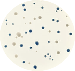
Figure 1. Original blue and white bacteria colonies in Petri dish.
Let’s imagine that we are working at the lab trying to optimize a new cloning protocol. We have dozens of Petri dish with transformed bacteria and we want to check and quantify the transformation efficiency. Each Petri dish will contain blue and white bacteria colonies, white ones will be the bacteria that have inserted our vector disrupting the lacZ gene that generates the blue color.
We want to take photos of the Petri dishes, transfer them to the computer and use a Python script to count automatically the number of blue and white colonies.
For example, we will analyze one image (Figure 1: ‘colonies01.png’) running the following command:
> python bacteria_counter.py -i colonies01.png -o colonies01.out.png
   30 blue colonies
   17 white colonies

Figure 2. Blue and white bacteria colonies are marked in red and green colors respectively as recognized by the Python script.
It will print the number of colonies of each type (blue and white) and it will create an output image (Figure 2: ‘colonies01.out.png’) where blue colonies are marked in red color and white ones in green.
Before showing the code I’ll do a few remarks:
- Code works quite well but it is not perfect, it fails to recognize 2 small white colonies and also groups other 2 small colonies with 2 bigger ones of the same color. Finally, the script counts 30 blue and 17 white colonies.
- One of the most tricky parts of the code are the color boundaries to recognize blue and white spots. These thresholds have been manually adjusted (with Photoshop help) before the analysis and they could change with different camera illumination conditions.
- White colonies are more difficult to identify because their colors are grayish and similar colors are in the blue colonies edges and background. For that reason, image colors are inverted previously to white colonies analysis for an easier recognition.
- It’s not AI (Artificial Intelligence). I’d call it better ‘Human Intelligence’ because the recognition algorithm thresholds are manually trained. If you are interested in AI and image recognition I can suggest to read the recent article in Nature about skin cancer classification with deep neural networks.
- I wanted to show a scientific application of image processing, but many other examples are available in internet: recognizing Messi face in a photo, classifying Game Boy cartridges by color…
And here is the commented code that performs the magic:
# -*- coding: utf-8 -*-
"""
Bacteria counter

    Counts blue and white bacteria on a Petri dish

    python bacteria_counter.py -i [imagefile] -o [imagefile]

@author: Alvaro Sebastian (www.sixthresearcher.com)
"""

# import the necessary packages
import numpy as np
import argparse
import imutils
import cv2

# construct the argument parse and parse the arguments
ap = argparse.ArgumentParser()
ap.add_argument("-i", "--image", required=True,
    help="path to the input image")
ap.add_argument("-o", "--output", required=True,
    help="path to the output image")
args = vars(ap.parse_args())

# dict to count colonies
counter = {}

# load the image
image_orig = cv2.imread(args["image"])
height_orig, width_orig = image_orig.shape[:2]

# output image with contours
image_contours = image_orig.copy()

# DETECTING BLUE AND WHITE COLONIES
colors = ['blue', 'white']
for color in colors:

    # copy of original image
    image_to_process = image_orig.copy()

    # initializes counter
    counter[color] = 0

    # define NumPy arrays of color boundaries (GBR vectors)
    if color == 'blue':
        lower = np.array([ 60, 100,  20])
        upper = np.array([170, 180, 150])
    elif color == 'white':
        # invert image colors
        image_to_process = (255-image_to_process)
        lower = np.array([ 50,  50,  40])
        upper = np.array([100, 120,  80])

    # find the colors within the specified boundaries
    image_mask = cv2.inRange(image_to_process, lower, upper)
    # apply the mask
    image_res = cv2.bitwise_and(image_to_process, image_to_process, mask = image_mask)

    ## load the image, convert it to grayscale, and blur it slightly
    image_gray = cv2.cvtColor(image_res, cv2.COLOR_BGR2GRAY)
    image_gray = cv2.GaussianBlur(image_gray, (5, 5), 0)

    # perform edge detection, then perform a dilation + erosion to close gaps in between object edges
    image_edged = cv2.Canny(image_gray, 50, 100)
    image_edged = cv2.dilate(image_edged, None, iterations=1)
    image_edged = cv2.erode(image_edged, None, iterations=1)

    # find contours in the edge map
    cnts = cv2.findContours(image_edged.copy(), cv2.RETR_EXTERNAL, cv2.CHAIN_APPROX_SIMPLE)
    cnts = cnts[0] if imutils.is_cv2() else cnts[1]

    # loop over the contours individually
    for c in cnts:

        # if the contour is not sufficiently large, ignore it
        if cv2.contourArea(c) < 5:
            continue

        # compute the Convex Hull of the contour
        hull = cv2.convexHull(c)
        if color == 'blue':
            # prints contours in red color
            cv2.drawContours(image_contours,[hull],0,(0,0,255),1)
        elif color == 'white':
            # prints contours in green color
            cv2.drawContours(image_contours,[hull],0,(0,255,0),1)

        counter[color] += 1
        #cv2.putText(image_contours, "{:.0f}".format(cv2.contourArea(c)), (int(hull[0][0][0]), int(hull[0][0][1])), cv2.FONT_HERSHEY_SIMPLEX, 0.65, (255, 255, 255), 2)

    # Print the number of colonies of each color
    print("{} {} colonies".format(counter[color],color))

# Writes the output image
cv2.imwrite(args["output"],image_contours)

 The didactic materials in this new section will be licensed as Creative Commons Attribution-NonCommercial.
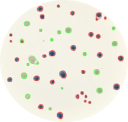

 Here I’ll summarize some Linux commands that can help us to work with millions of DNA sequences from New Generation Sequencing (NGS).